
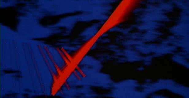
Stone detected bouncing off rocky terrain at center
In the 1987 film Predator, the movie at time 1:31:30 shows what the Predator sees through his mask throughout what appears to be a calculation that predicts the location of Dutch hiding.
Although the animation appears a bit cryptic, it is fairly easy to recognize that the calculation is essentially concerned with the trajectory of a stone that was thrown by Dutch at time ~1:31:00.
Although most people think that the animation concerns the trajectory of the Predator's ballistic, in reality the calculation is that of the reverse trajectory of the stone that Dutch threw.
The Predator then, can calculate the reverse trajectory of the stone using this data:
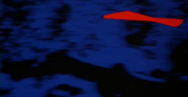
The first datum is the first bouncing of the stone in the following snapshot:
Further successive bounces are detected as the stone falls down from the rocky terrain. This allows the Predator to calculate y0.
If you look carefully at time 1:31:15, the Predator detects a bouncing stone angle of ~-2π/3 off the rocky terrain.
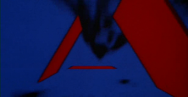
The next datum calculated will then be the reverse launch angle at the first bouncing point, which will be approximately equal to 2π/3 - since the bounce off the rock angle and the strike angle have to be complementary. This is shown as the normal to the reverse launch at the bouncing point in the following figure:
The Predator now has all the data it needs to solve the stone's reverse trajectory, as initial value problem: {dy/dt=f(t,y);y(t0)=y0}.
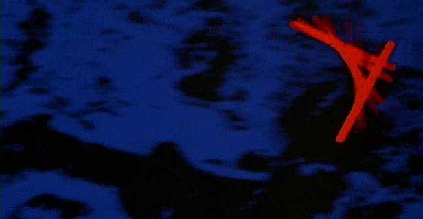
The next sequence of red lines appear to be tangents to the reverse stone trajectory:

Let's see if we can now numerically approximate the problem's solution, using the classic Runge-Kutta Method and Maple:
>with(plots):
>theta:=2*Pi/3;#rock striking angle or reverse launch angle
>v:=20;#m/s - vertical component of velocity - gotten through stone bouncing off
rock data
>g:=9.81;#m/s^2 #assumed, measured prior by Predator for Earth
>x:=t->v*cos(theta)*t;#horizontal displacement. Assumed known in theory by
Predator
>y0:=10;#m - calculated from stone falling off rocky cliff. Height of reverse
launch
>y:=t->y0+v*sin(theta)*t-1/2*g*t^2;#vertical displacement. Law known by
Predator
>at:=plot(y(t),t=0..2.5):# theoretical vertical displacement
>f:=unapply(diff(y(t),t),t,y);#initial value problem to be solved
>RKP:=proc(yn,tn,h)#Runge Kutta 4 method for Initial Value Problem for f
>local k1,k2,k3,k4;
>k1:=f(tn,yn);
>k2:=f(tn+1/2*h,yn+1/2*h*k1);
>k3:=f(tn+1/2*h,yn+1/2*h*k2);
>k4:=f(tn+h,yn+h*k3);
>yn+1/6*h*(k1+2*k2+2*k3+k4);
>end:
>h:=0.1;#step size for RK4 method
>RKPT:=proc(y0,t0,h)#Runge-Kutta 4 reverse trajectory predictor for stone
>local T,tn,yn,n;
>yn:=y0;tn:=t0;
>T:=[[tn,yn]];
>for n from 1 to floor(abs(3/h)) do
>tn:=tn+h;yn:=RKP(yn,tn,h);
>T:=[op(T),[tn,yn]];
>od;
>T;
>end:
>t0:=2.5;#final time (we are calculating in reverse, so this is reverse launch time)
>PT:=RKPT(y(t0),t0,-h):#Projected reverse trajectory of stone
The process appears to converge at a rocky crevice, close to where Dutch is hiding:
We can now compare the theoretical trajectory with the projected one:
>p:=plot(PT,style=point,symbol=cross,color=blue):
>display({p,at});#projected by RK4 combined with theoretical trajectory
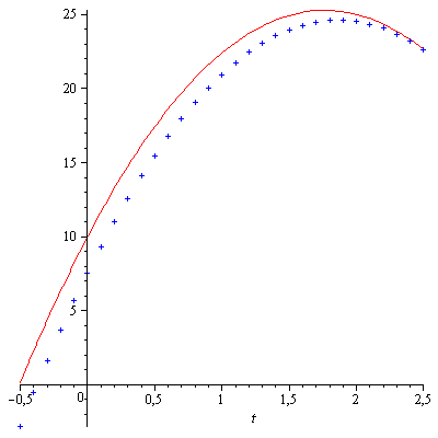
The red line animation therefore represents the k constants in RK4 at discrete time intervals, which are the tangents of the trajectory at those time intervals. Note that as in the movie, there is a slight miss, but not by much.