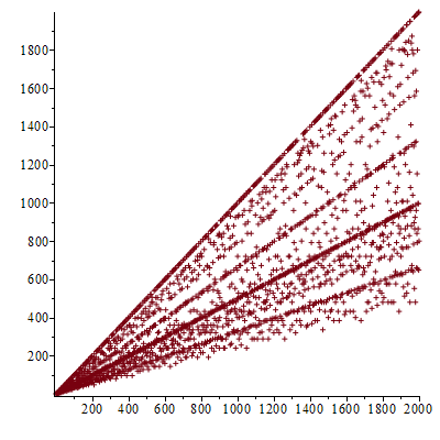
While looking at the wiki page for Euler's totient function φ, we notice that Wiki has a graph of φ(n) versus n on the upper right side of the page, so we explore this result with Maple:
>with(numtheory):
>with(plots):
>lim:=2000;
>liste:=[seq([n,phi(n)],n=1..lim)]:
>p:=plot(liste,style=point, symbol=cross):
>display(p);

One notices that the graph displays some obvious "trends" or lines where many points accumulate, so the author tried to figure out the approximate functions which describe those trends: First, it's obvious that the upper line is the line f(x)=x-1, since φ(p)=p-1, for p prime. Hence the highest line consists of primes.
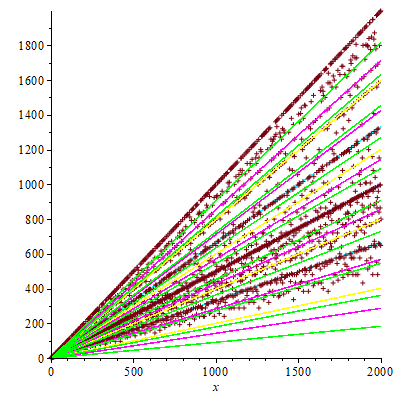
The author fitted the rest of some lines, based on the rough heuristic that the next major trend looks like f in F1={x/2}, and continuing in the obvious way with f in F2={x/3,2*x/3}, F3={x/5,2*x/5,3*x/5,4*x/5}, F4={x/7,2*x/7,3*x/7,4*x/7,5*x/7,6*x/7}, F5={x/11,2*x/11,3*x/11,4*x/11,5*x/11,6*x/11,7*x/11,8*x/11,9*x/11,10*x/11}, etc.
>p:=plot(x-1,x=0..lim,color=black):
>q:=plot(x/2,x=0..lim,color=blue):
>r:=plot({x/3,2*x/3},x=0..lim,color=cyan):
>s:=plot({x/5,2*x/5,3*x/5,4*x/5},x=0..lim,color=yellow):
>t:=plot({x/7,2*x/7,3*x/7,4*x/7,5*x/7,6*x/7},x=0..lim,color=magenta):
>u:=plot({x/11,2*x/11,3*x/11,4*x/11,5*x/11,6*x/11,7*x/11,8*x/11,9*x/11,10*x/11},x=0..lim,color=green):
>display({p,q,r,s,t,u});
The resulting graph combined with that of the totient:
So the author set forth to ask this question in the newsgroup sci.math. He includes here Gerry Myerson's reply for completeness:
"As you noticed, if p is prime then φ(p) = p - 1, so there will be points just below y = x for each prime. But the primes are few and far between once you get to large values of x, so in a sense those points are not really very dense at all. But you also get close to y = x if n = p q with p and q both large primes. In fact, if n is any number all of whose prime factors are large then phi(n) will be relatively close to n.
If n = 2 p or n = 4 p or n = 8 p or ... where p is an odd prime then phi(n) is just less than n 2, so that gives you points near y = x 2. Numbers of the form 3 p, 9 p, 27 p, etc., give points near y = 2 x 3. Numbers 6 p, 12 p, 18 p, 24 p, 36 p, 48 p, 54 p, 72 p, etc., give points near y = x 3...."
Now let's dissect Gerry's answer: The highest line is indeed the line f(x)=x-1. Then:
For n=2kp, k in N, p odd prime:
φ(n)=φ(2kp)=2kp(1-1/2)(1-1/p)=(n/2)(p-1)/p. For large p,
(p-1)/p ~ 1, hence also for large n, φ(n)~n/2, consequently these numbers follow
approximately the trend f(x)=x/2.
For n=3kp, k in N, p prime > 3:
φ(n)=φ(3kp)=3kp(1-1/3)(1-1/p)=(2n/3)(p-1)/p. For large p,
again (p-1)/p ~ 1, hence also for large n, φ(n) ~ 2 n/3, consequently these numbers
follow the trend f(x)=2*x/3.
For n=2k3lp, k,l in N, p prime > 3:
φ(n)=2k3lp(1-1/2)(1-1/3)(1-1/p)=(n/2)(2/3)(p-1)/p=(n/3)(p-1)/p,
hence again for large n, φ(n) ~ n/3, consequently these numbers follow the trend
f(x)=x/3.
Let's do some more:
For n=5kp, k in N, p prime > 5:
φ(n)=5kp(1-1/5)(1-1/p)=(4n/5)(p-1)/p, hence for large n, φ(n) ~
4n/5, consequently these numbers follow the trend f(x)=4*x/5.
For n=2k5lp, k,l in N, p prime > 5:
φ(n)=n(1-1/2)(1-1/5)(1-1/p)=(2n/5)(p-1)/p, hence the trend f(x)=2*x/5.
For n=3k5lp, k,l in N, p prime > 5:
φ(n)=n(1-1/3)(1-1/5)(1-1/p)=(8n/15)(p-1)/p, hence the trend f(x)=8*x/15.
For n=2k3l5mp, k,l,m in N, p prime > 5:
φ(n)=n(1-1/2)(1-1/3)(1-1/5)(1-1/p)=(4n/15)(p-1)/p, hence the trend f(x)=4*x/15.
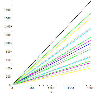
Here is the graph with all the trends for n=2k3l5m7qp, k,l,m,q in N U {0}, p prime > 7:
Now let's look at some actual counts:
> margin:=2;
> trends:=16;
> c:=array(1..trends);
> for n from 1 to trends do
> c[n]:=0;
> od:
> for n from 1 to lim do
> t:=phi(n);
> if abs(t-n)<=margin then
> c[1]:=c[1]+1;
> elif abs(t-n/2)<=margin then
> c[2]:=c[2]+1;
> elif abs(t-n/3)<=margin then
> c[3]:=c[3]+1;
> elif abs(t-2*n/3)<=margin then
> c[4]:=c[4]+1;
> elif abs(t-2*n/5)<=margin then
> c[5]:=c[5]+1;
> elif abs(t-4*n/5)<=margin then
> c[6]:=c[6]+1;
> elif abs(t-4*n/15)<=margin then
> c[7]:=c[7]+1;
> elif abs(t-8*n/15)<=margin then
> c[8]:=c[8]+1;
> elif abs(t-2*n/7)<=margin then
> c[9]:=c[9]+1;
> elif abs(t-3*n/7)<=margin then
> c[10]:=c[10]+1;
> elif abs(t-4*n/7)<=margin then
> c[11]:=c[11]+1;
> elif abs(t-6*n/7)<=margin then
> c[12]:=c[12]+1;
> elif abs(t-8*n/35)<=margin then
> c[13]:=c[13]+1;
> elif abs(t-12*n/35)<=margin then
> c[14]:=c[14]+1;
> elif abs(t-16*n/35)<=margin then
> c[15]:=c[15]+1;
> elif abs(t-24*n/35)<=margin then
> c[16]:=c[16]+1;
> else ;
> fi;
> od:
> p1:=plot([[1,0],[1,evalf(c[1]/lim)]],color=black):#x-1
> p2:=plot([[2,0],[2,evalf(c[2]/lim)]],color=blue):#x/2
> p3:=plot([[3,0],[3,evalf(c[3]/lim)]],color=cyan):#x/3
> p4:=plot([[4,0],[4,evalf(c[4]/lim)]],color=cyan):#2*x/3
> p5:=plot([[5,0],[5,evalf(c[5]/lim)]],color=yellow):#2*x/5
> p6:=plot([[6,0],[6,evalf(c[6]/lim)]],color=yellow):#4*x/5
> p7:=plot([[7,0],[7,evalf(c[7]/lim)]],color=magenta):#4*x/15
> p8:=plot([[8,0],[8,evalf(c[8]/lim)]],color=magenta):#8*x/15
> p9:=plot([[9,0],[9,evalf(c[9]/lim)]],color=green):#2*x/7
> p10:=plot([[10,0],[10,evalf(c[10]/lim)]],color=green):#3*x/7
> p11:=plot([[11,0],[11,evalf(c[11]/lim)]],color=green):#4*x/7
> p12:=plot([[12,0],[12,evalf(c[12]/lim)]],color=green):#6*x/7
> p13:=plot([[13,0],[13,evalf(c[13]/lim)]],color=grey):#8*x/35
> p14:=plot([[14,0],[14,evalf(c[14]/lim)]],color=grey):#12*x/35
> p15:=plot([[15,0],[15,evalf(c[15]/lim)]],color=grey):#16*x/35
> p16:=plot([[16,0],[16,evalf(c[16]/lim)]],color=grey):#24*x/35
> with(plots):
> display({p1,p2,p3,p4,p5,p6,p7,p8,p9,p10,p11,p12,p13,p14,p15,p16});
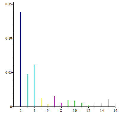
P(n=prime)=c[1]/lim ~ 0.1525
Prime number theorem gives: P(n=prime)=1/log(lim) ~ 0.1315633249
Running the same program for lim=10000, we find thus:
P(n=prime)=c[1]/lim ~ 0.1231
Prime number theorem gives: P(n=prime)=1/log(lim) ~ 0.1085736205
In a sense, the above probabilities represent the "density" of the trend lines in the graph of φ for the space [1..lim].
For a slightly deeper analysis, consult this answer on math.StackExchange.