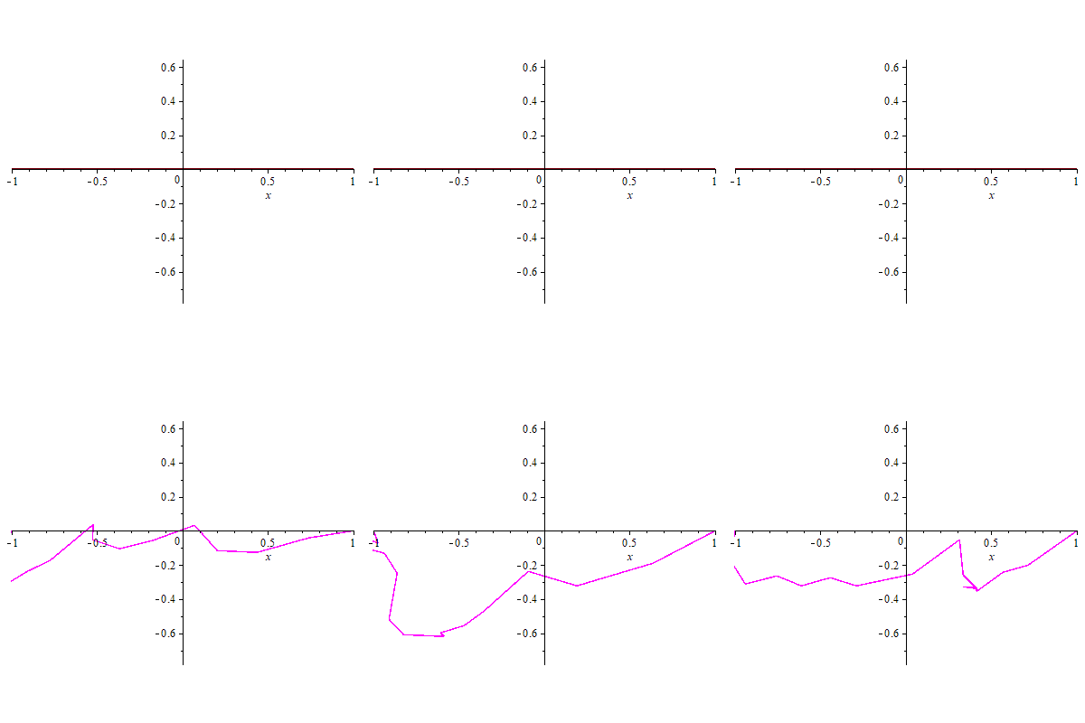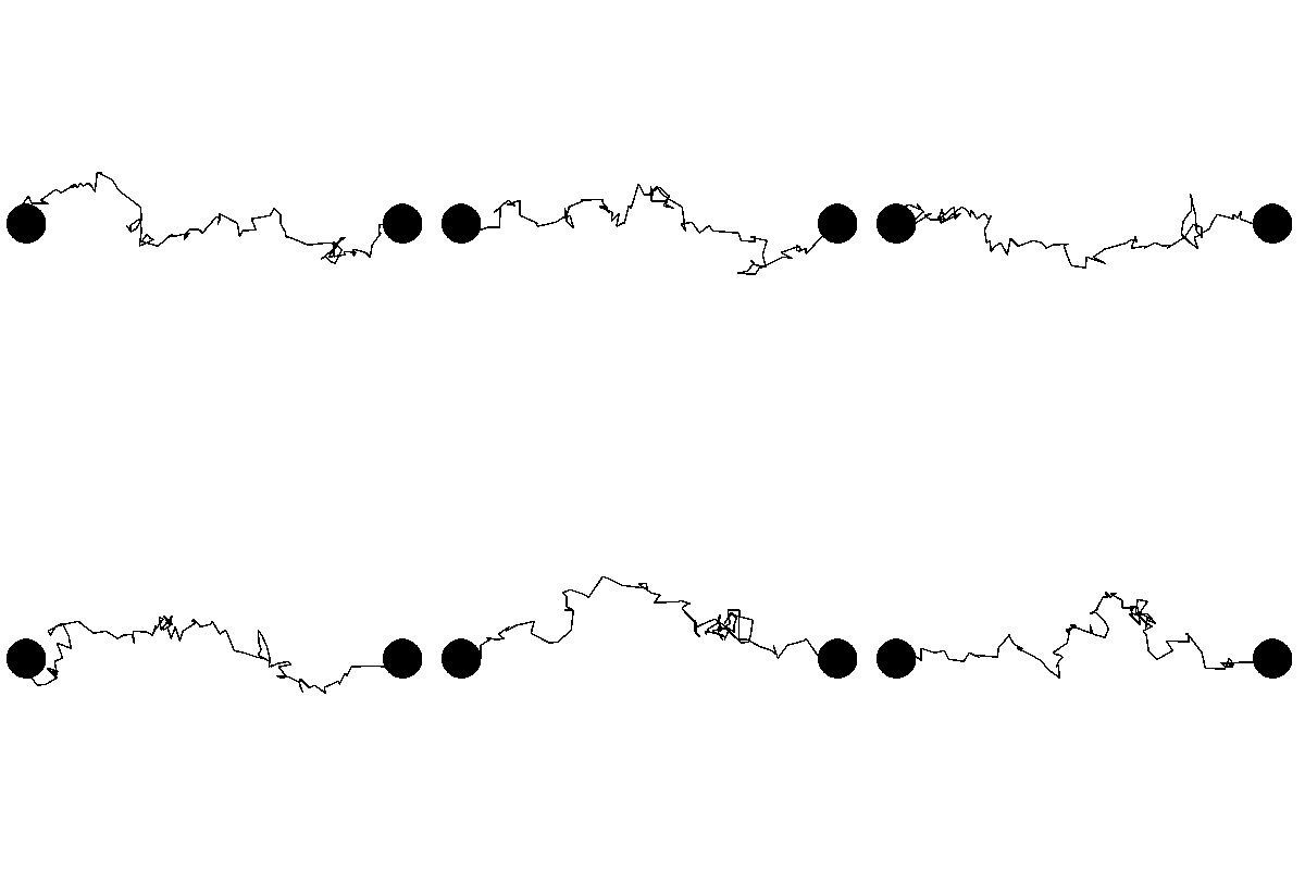
Simulation of electric spark between two poles (-1,1), as a Lichtenberg fractal figure
A Lichtenberg figure is a fractal[1] figure whose pattern is to be found in nature. Some examples are: Vein shapes, tree branches, neurons (brain and bodily), trachea shapes, electric sparks (from Tesla coils, Van de Graaff generators, Lightning, etc).
The pattern is also found in the breakup of (thick) dielectric material, when high voltage is applied at opposite ends. The figure can be 2D or 3D, branching or not. Branching, when multiple terminals are employed, single branch if only two poles are employed.
It is also found upon the breakup of non-elastic or very slightly elastic materials, such as when glass, crystal or concrete, when they break under tension[2].
It is similar to Brownian motion which characterizes the motion path of particles in fluids and the overall path a photon takes starting from the core of a star until it reaches its surface[3].
A Random walk is a special case of Brownian motion with constraints on the change of direction.
The overall path of a single branch is characterized as being linear piecewise and is therefore not differentiable at the points which the path changes direction. There are only a finite number of points where the path changes direction[4].
Let's try some Maple code:
>restart;
>with(plots):
>p:={};cdet:=1/10;
>L:=proc(z1,z2,dis)
>local l,nz,midx,midy;global p,cdet;
>if dis
> p:=p union {plot([[Re(z1),Im(z1)],
[Re(z2),Im(z2)]],x=-1..1,scaling=constrained,color=magenta)};
>else
> midx:=evalf((Re(z1)+Re(z2))/2);
> midy:=evalf((Im(z1)+Im(z2))/2);
> midx:=midx + (RandomTools[Generate](float(range=0..1,digits=2))-1/2)*dis;
> midy:=midy + (RandomTools[Generate](float(range=0..1,digits=2))-1/2)*dis;
> nz:=evalf(midx+midy*I);
> L(z1,nz,dis/2);
> L(nz,z2,dis/2);
>fi;p;
>end:
>display(L(-1,1,1.3));

An alternate simulation using Robert Israel's code:
>N := 100; c := 0.2; nframes:= 20;
>plots[display]([BB, plottools[disk]([0, 0], 0.5e-1, colour = black), plottools[disk]([1, 0], 0.5e-1, colour = black)], scaling = constrained, axes = none);
