Google Scholar can be used to construct a metric which can show
the relative "merit" of scientists in their corresponding fields of research, based
on the work they've done.
Assuming that an author's name is unique (which is not always the case), one can
construct a characteristic publication number or a publication eignevalue
for a given author, say "john doe", as follows:
Enter "author:j-doe" in the Google scholar field and press "Search".
a0=number of results for this author, shown on the upper right
hand.
a1=number of citations under the first result. Click on these
citations. A new window opens.
a2=number of citations under the first result. Click on these
citations. A new window opens.
...
Repeat, until first result shows no citations or the sequence falls into a
cycle.
The publication eigenvalue for this author then, can be the number C(john doe),
which has the continued fraction expansion:
C(john doe)=[a0;a1,a2,...,an,...].
To simplify the ordering which is present in the set {C(x):x\in author}, without
loss of generality we can set a0=1 and look instead at the number:
C(john doe)=[1;a0',a1',a3',...,an',...],
with an-1'=an, which maps the set {C(x):x\in author} into the
interval (1,∞).
Note that in this case, supx{C(x):x\in author}=∞ and
infx{C(x):x\in author}=1.
Adding a citation entry a>0 to an existent continued fraction expansion of C(x),
can make C(x) either larger or smaller, depending on where a is added and the number of
citations at level n[18].
Specifically:
[1;a1,a2,a3,...,an,a]<[1;a1,a2,a3,...,an],
if n odd,
[1;a1,a2,a3,...,an,a]>[1;a1,a2,a3,...,an],
if n even
[1;a1,a2,a3,...,an+a]<[1;a1,a2,a3,...,an],
if n odd.
[1;a1,a2,a3,...,an+a]>[1;a1,a2,a3,...,an],
if n even.
The main "weight" of the number C(x) will then be carried by the term a1,
which is the number of publications of author x and which provides a good approximation
of C(x), as C(x)~C2(x)=1+1/a1, which is fairly reasonable.
The formal definition of C(x) is slightly more involved, mainly because one
needs to define it uniquely. Here's then the formal definition:
Let x be the name of an author in Google Scholar.
Search on x gives rise to a1 results.
Each result gives rise to a2,k citations, indexed by k.
Each of those results gives rise to a3,l citations, indexed by l, and
so on.
Define C(x)=[a0=1;a1,...,an,...], with:
a1=supk{a1,k},a2=supl{a2,l},...,an=supw{an,w}.
It can now be seen that the definition above gives rise to a unique number
C(x), as in the first definition for "john doe", above, because the suprema are taken
over finite sets indexed by k,l,m,...,w.
A Metric Based On Google Scholar
The definition above gives rise to the metric: d(x,y)=|C(x)-C(y)|. Let's
verify the metric's fundamental properties:
d(x,y)≥0: Follows from the definition of |.|.
d(x,y)=0 <=> x=y: Let
C(x)=[a0=1;a1,a2,...,an] and
C(y)=[b0=1;b1,b2,...,bm]. If x=y, then
m=n and C(x)=C(y), so |C(x)-C(y)|=d(x,y)=0.
Conversely, if d(x,y)=|C(x)-C(y)|=0 and m=n, then ai=bi, for
all i \in {0,1,2,...,n}, which happens if x=y. If m=/=n, then the simplest case is
[1;a]=[1;b,c], which gives: a=b-1/c, which forces c=1 because a and b are naturals,
therefore c=1 and b=a-1. In other words, in the simplest case y has 1 less
publication than x, but also one more citation. In general this may also happen if y
has one less citation at level n and one more at level n+1. These are rare cases, and
if they are excluded, then x=y.
For any w, d(x,y)=|C(x)-C(w)+C(w)-C(y)|≤|C(x)-C(w)|+|C(w)-C(y)|=d(x,w)+d(w,y),
by the triangle inequality for |.|.
It is clear that a person with no publications, will have a characteristic number
equal to infinity and the more publications an author has, the closer C(x) is to 1.
This gives rise to a tempered distribution, and then one can define the publication
percentile P(x) of a scientist x in this distribution to be: P(x)=100/C(x).
Fixing t=now(18/11/2010) and omitting the term a0=1, let's then see these
numbers for some scientists:
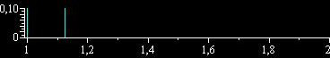
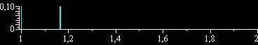
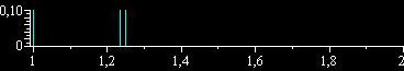
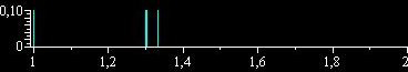
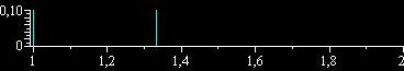
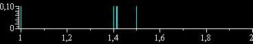
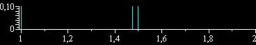
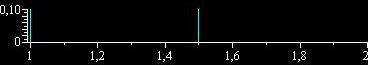
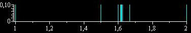
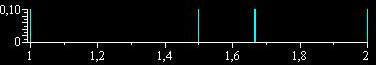
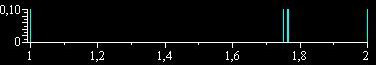
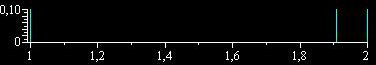
We can now define the Google Scholar Eigenspectrum of the author x to be the
sequence of convergents for C(x),
Cn(x)=[a0=1;a1,a2,...,an-1].
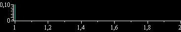
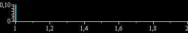
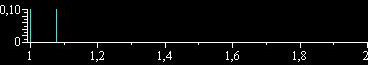
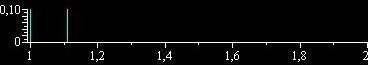
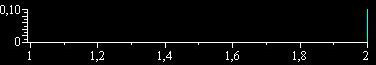
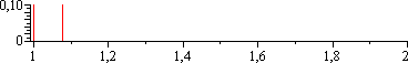
The spectra of some authors are shown below. The dominant spectral line for each
author lies approximately at
C2(x)=a0+1/a1=1+1/a1. These spectra give
you a rough idea of the colossal amount of work the corresponding authors have done in
their fields.
Euler proved that whenever the sequence of the associated continued fraction is
periodic, C(x) will equal a certain quadratic irrational ζ
of the form (P+sqrt(D))/Q. We find this ζ for this author.
First we program some Maple code to calculate continued fractions.
> L2C:=proc(L)
> local l,c,n;
> l:=nops(L);c:=0;
> for n from 1 to l do
> c:=1/(c+L[l-n+1]);
> od;
> c;
> 1/c;
> end:
The above proc, takes as input a list of the form:
>L:=[a0=1,a1,a2,a3,a4,...];
and calculates the corresponding continued fraction.
Consider then the simplest periodic continued fraction, with a period 2 block p:
[a1;a2,a1,a2,...,a1,a2,...].
What does it mean for this continued fraction to be periodic? It means
exactly:
p=a1+1/(a2+1/p) (1)
Equation (1) translated into continued fraction notation, is:
p=[a1;a2,p] (2)
Equation (2) translated into Maple notation, is:
L2C([a1;a2,p])=p
The last equation can be solved quickly with Maple.
> eq:=L2C([a1,a2,p])=p;
> sol:=solve(eq,p);
The above gives two solutions. For this author the continued fraction of works and
citations (including the initial 1) is:
L=[1;13,10,4,17,3,17,3,17,3,...]. Therefore, we can recover the periodic part,
as:
> zeta:=simplify(zeta0);
> conj:=denom(zeta)-2*op(denom(zeta))[2];#get rid of roots on denominator!
> zetan:=expand(numer(zeta)*conj);
> zetad:=expand(denom(zeta)*conj);
> zeta:=zetan/zetad;
And ζ=906371/842062-(1/2526186)*2805(1/2), so the Publication
Eigenvalues for this author, as a function of t=now, are ζ and ζ*, which are
Quadratic Irrationals[32].
This equation then, is something like a characteristic equation or
eigenequation for this author and the left part of the equation is something
like a publication eigenfunction for this author as a function of this author's
publications at the current time. As more works are published and more citations are
shown, it is obvious that this characteristic equation changes as a function of time.
It is a useful exercise for the reader to calculate the characteristic equation of
other authors, higher on the table, above.
The Eigensignal of an Author
The convergents of C(x), are {Cn(x)}, n\in N, and they can be calculated
with Maple:
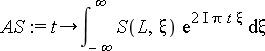
If δ is the Dirac Delta, the Google Scholar Publication Eigenspectrum of an
author x shown on the above table then, is the convergent pulse train or
Dirac Comb:
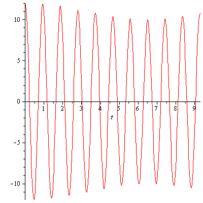
The Google Scholar Publication Signal or Publication Eigensignal of an
author in the time domain then, will be the Inverse Fourier Transform of the author's Eigenspectrum:
If C(x) is rational the sum will consist of a finite number of terms and hence the
Eigensignal will be periodic in the time domain[12]. If C(x) is a quadratic irrational the sum
will consist of infinitely many terms and the eigensignal will not be periodic in the
time domain.
Let's calculate the real and imaginary components of the eigensignal for this author
with Maple, by considering an approximation with the periodic part of C(x) repeating 4
times:
> L:=[1,13,10,4,17,3,17,3,17,3,17,3];
> S:=proc(L,n)
> local i;
> add(Dirac(xi-C(L,i)),i=1..nops(L));
> end:
>a0:=2/T*Int(rexpr(t),t=0..T):
>a:=n->2/T*Int(rexpr(t)*cos(2*Pi*n*t/T),t=-T/2..T/2):
>b:=n->2/T*Int(rexpr(t)*sin(2*Pi*n*t/T),t=-T/2..T/2): #evaluates to 0
These evaluate to functions of the convergents of C(x)[13].
If C(x) is a quadratic irrational, the author's Google Scholar Eigensignal will be
"almost" periodic, with a minimal period T=1/Cn(x) which is with Maple:
> T:=1/C(L,nops(L));#find minimal period! (which we used in calculations
above)
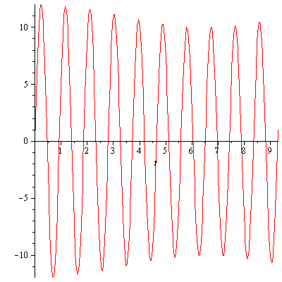
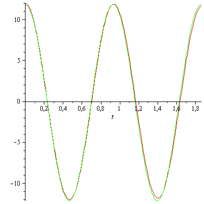
Now we can construct a Fourier Series approximation for the real Eigensignal with
Maple:
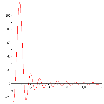
Real part of author's Publication Eigensignal (red) and Fourier Series approximation
F12(x,t) (green)
The harmonics of the author's real Eigensignal will then be an and
the amplitude of the harmonics will be given as cn=|an|.
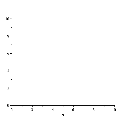
The author's Harmonic Spectrum with up to 10 harmonics is shown below.
Harmonic Spectrum for this author's Eigensignal with up to 10 harmonics
(a1~11.95)
The 0-th harmonic a0 (dc-term) is the red line (almost supressed). The
amplitude of the dominant harmonic (green), which corresponds to the
dominant spectral line shown on the author's Eigenspectrum on the table above, is
|a1|~11.95 and the author's Eigensignal broadcasts at a frequency
f=1/T=C(x)~1.082 Hz.
We now have a Fourier Series approximation. Let's recover the Google Eigenspectrum
from it.
Recovered Eigenspectrum for this author from F12(x,t)
The above is an approximation of the Google Scholar Eigenspectrum for this author.
The function jumps very hight exactly at the convergents Cn(x) and in
particular at C2(x):
> evalf(SSS(C(L,2)));
119.3746313
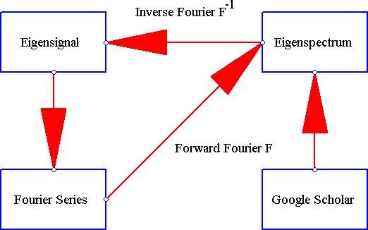
We therefore have verified the commutativity in the following diagram:
Commutative diagram for Eigenspectrum, Eigensignal and Fourier Series
The publication Eigensignal's minimal period is roughly the time between two
adjacent publications. For this author:
Accordingly, one can now define a x author's blue-shift relative to another
author y, via the Google Scholar Metric, as d(x,y)=|C(x)-C(y)|. For example:
The author's advisor is blue-shifted 0.03090244910 more than the author. x more
blue-shifted than y means x has worked harder than y. Notice how high are the
blue-shifts of the big guns in Mathematics.
Alternatively one may define an author's red-shift relative to unity. For
example:
The author's advisor is 0.04544744665 and the author is 0.07634989575 red-shifted
away from unity. Smaller red-shifts mean more work.
Notes/References
The sequences were extracted on the date of publication (18/11/2010) and
consequently they may be different on the date the reader reads this article. To
calculate the continued fraction sequence, the author entered the author's names in
Google Scholar, as "author:j-a-doe", where "j" and "a" are the initials of the
author's first and middle name. When this didn't work, for example when the list of
references included other people, the full name was entered as "author:john-doe".
When even this didn't work, the name was entered as "author:john-a-doe". If you are
listed above and disagree with your sequence, send this author a more appropriate
sequence which can be verified via Google Scholar. The spectra tables are not meant
to be exhaustive. Only a small selection of scientists is presented. If you are not
listed above and you have a Google Scholar publication history, or you want to
nominate someone else for inclusion, you can send this author your full name and a
home page link or the name of the nominee and he will add a corresponding entry to
both tables.
Rational or quadratic irrational.
Length of non-periodic block in the author's continued fraction.
Length of periodic block in the author's continued fraction.
This author considers Oppy's work to be of fundamental historical importance
since with his work humanity graduated as a nuclear power. Accordingly, this man is a
major critical point in the development of human scientific intelligence. An
author's x Eigenspectrum can be labelled relativistic when the red-shift of x
is less than that of Oppy. In symbols: Rel(x) <=> C(x)≤C(Oppy). For example,
the authors above Oppy all have relativistic eigenspectra.
Can you think what rational or quadratic irrational imply in terms of publication
events for the corresponding authors?
If C(x) is rational then the number of spectral lines is finite, hence the sums
in a0 and an are finite. If C(x) is a quadratic irrational,
because Cn(x) converges very fast, the Eigenspectrum can be approximated
by a finite pulse train, consisting of the first m convergents
Cm(x), in which case a0 and an can again be
approximated by a finite summation. In the subsequent Maple approximation example m
is the cardinality of the sequence list.
The Eigenspectrum can be characterized as rare or strange in that
it displays two spectral lines which are widely separated. It is instructive
for the reader to try to identify the root cause of this phenomenon.
This means for example, that this author at the beginning was writing
approximately 1 paper every 11 months, which checks pretty well with the publication
dates of his papers on his Mathematics page. For an author
x, his average publication period will be given roughly as
T0~1/Cn(x).
The author's father is found having a lower rating than the author, which is
rather silly and highly contradictory. The discrepancy can be partially explained by
noticing that, first, his father's field was Applied Mathematics in Civil
Engineering: Theory of Elasticity, which is a very rare field and second, that his
father was a professor for only 5 years before leaving this post. The sequence was
generated by his Ph.D.. Additionally, Google Scholar ignores several of his
other publications, such as these which are in Greek Engineering journals. For
details about these, consult the author's notes in his father's biography.
This is fairly reasonable because citations detract/add importance to the main
publications from the author and assign it to the authors of the citations depending
on their nesting level. If one wants, one can arrange C(x) to have its convergents be
monotone decreasing using appropriate functions of the an instead of the
terms an themselves.
The author's general surgeon. Field: Medicine.
Has helped with the author's research on Tetration.
Has compiled a colossal amount of computational and mathematical data on his web
site.
The most prolific author in the area of Complex Dynamical Systems.
Has compiled a colossal amount of light and engineering data on his web
site.
Has compiled a colossal amount of light-engineering data.
The main resonance line in the Eigenspectrum of the author's father corresponds
roughly to the 436nm blue triple line in Mercury's spectrum emitted by the High Pressure Mercury Vapor Lamp, which played
an important role in the scientific development of the author.
The eigenspectra of the metal ratios curiously contain resonance lines which
match actual lines in their real
spectra.
The signals are not very accurate because the duration of each frame in animated
.gifs needs to be an integral multiple of 1/100 sec, while the actual durations after
calculation are seen to be decimal multiples of 1/100 secs for the two authors
shown.
Field: Light-engineering.
Professor at the University of Crete. Served as advisor for several of the
author's papers.
Note that Q|(P2-D):
>Pn:=numer(zeta);
>Q:=denom(zeta);
>Dr:=op(2,Pn)^2;
>P:=op(1,Pn);
>(P^2-Dr)/Q;
292677.