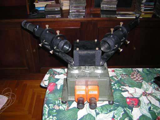
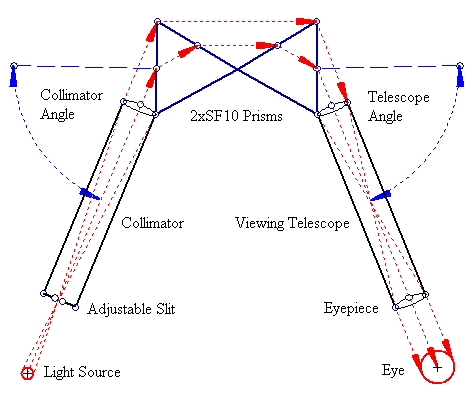
The Phasmatron Spectroscope. It was built in 1998 and cost €1,173+2x300(2x60x60x60 SF10 prisms).
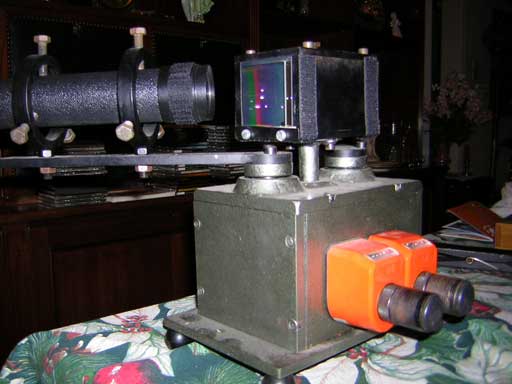
| Viewer | 8-24 x D=40mm |
| Collimator | D=50mm |
| Dispersive Medium | 2xSF10 Schott Equilateral Prisms, D=60x60x60mm |
| Adjustable slit | Spindler & Hoyer 0-3mm |
| Angle Readers | ± 90° from Normal of Prism Housing Dome |
| dn/dλ | 1.2702*10-5/A (Sodium D Light) |
| Resolution Δλ | 0.3866148 A (Sodium D Light) |
| Resolving Power R | 15242.4 (Sodium D Light) |
| dE/dn | 3.9724624 rad (Sodium D Light) |
| Dispersion dE/dλ | 5.04582*10-5 rad/A (Sodium D Light) |
| Spectrum Angular Width ΔE | 13.42°-16.84° |
| Weight |
35 kg |
| Light Type | Visible Spectrum Section | Spectral Distribution |
| [1]: Triphosphor fluorescent spectrum section on the area of the mercury yellow lines and the mercury green line at 8x. Compare with spectrum [1.3.4] taken with the smaller amici spectroscope. |  |
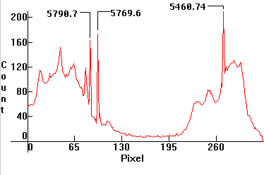 |
| [2]: Triphosphor fluorescent spectrum section on the area of the Europeum red fluorescence line and mercury yellow lines at 20x. Compare with [1.3.4] taken with the smaller amici spectroscope. |  |
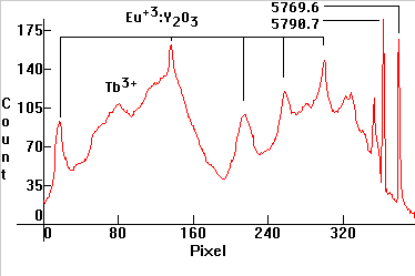 |
| [3]: Triphosphor fluorescent spectrum section on the area of the mercury green line at 16x, showing terbium fluorescence around the line. Compare with [1.3.4] taken with the smaller amici spectroscope. |  |
 |
| [4]: Triphosphor fluorescent spectrum section on the area of the mercury blue-green line at magnification of 16x, showing terbium fluorescence around the line. Compare with [1.3.4]. |  |
 |
| [5]: Triphosphor fluorescent spectrum section on the area of the mercury blue-green line at magnification of 24x. This is the same as [4], enlarged. |  |
 |
| [6]: Triphosphor fluorescent spectrum section of the area of the mercury blue line at magnification of 8x. This is equivalent to a low pressure mercury line at 436nm. |  |
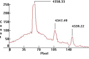 |
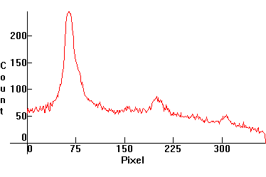
| [7]: High Pressure Mercury spectrum section of the area of the mercury blue line at magnification of 8x. This is the same area as [6]. Note self-absorption and thermal broadening of the blue Mercury line. | 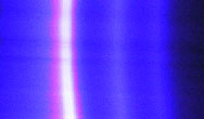 |
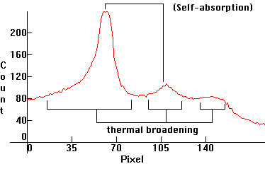 |
| [8]: Triphosphor fluorescent spectrum section of the area of the mercury blue line at magnification of 24x. This is again equivalent to a low pressure mercury line at 436nm. | 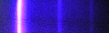 |
 |
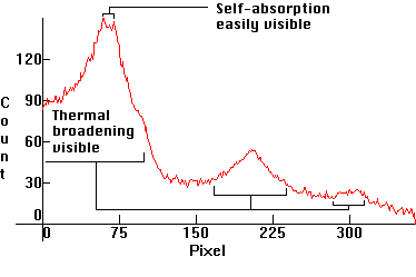
| [9]: The high pressure blue Mercury line at 24x. This is the same area as [8]. Self-absorption and thermal broadening are now easily visible. Photographs [8] and [9] are pushing the spectroscope to its limits. | 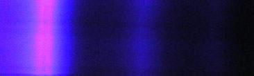 |
 |
| [10]: Portion of the Solar spectrum between the Hydrogen C=Ha and Sodium D lines. D lines resolve at 8x. | 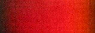 |
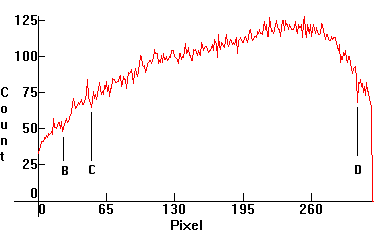 |
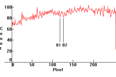
| [11]: Zoom on the Sodium D line, above at 24x. The D1/D2 absorption doublet is clearly visible. |  |
 |
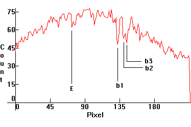
| [12]: Portion of the Solar spectrum around the iron E line, with Magnesium b1/b2/b3 lines visible. |  |
 |
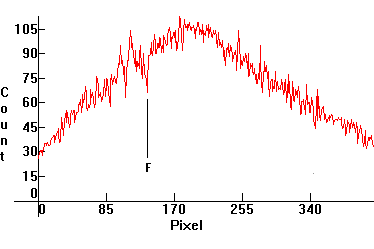
| [13]: Portion of the Solar spectrum around the F=Hb line. | 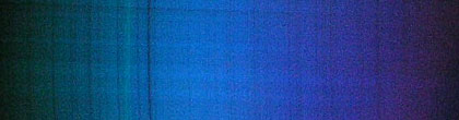 |
 |
| [14]: Section of the spectrum from a low pressure Sodium discharge at 8x taken while a high pressure Sodium lamp was warming up, and while mercury was still participating in the discharge. | 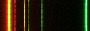 |
 |
| [15]: Same as [14], at 24x. The low intensity deep orange lines at (*) on this photo (approximately at the center of the photo) and on [14] are ghosts/artifacts of the Sodium D1/D2 lines. | 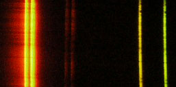 |
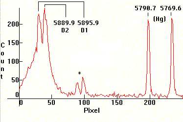 |
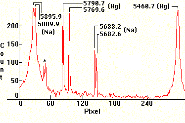
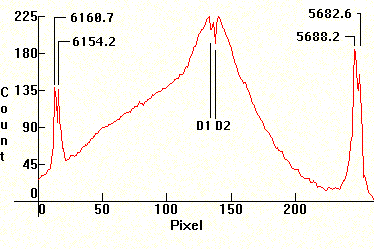
| [16]: Portion of the spectrum from a low pressure Sodium discharge. Besides the D1/D2 doublet two more Sodium doublets, a red one to the left and a green one to the right are visible. The (*) lines are ghosts, as in [14]/[15]. | 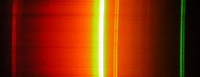 |
 |
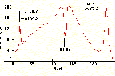
| [17]: Same as above, but with pressure increasing. The D1/D2 doublet is starting to self-absorb and emit light on the neighborhood of D1/D2 wavelengths (display of "wings"). | 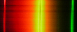 |
 |
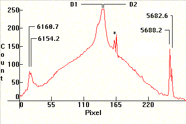
| [18]: Same as above, but with pressure still higher. The D1/D2 doublet has completely reversed itself and self-absorption is now clearly visible. The green Sodium doublet also displays some thermal broadening. | 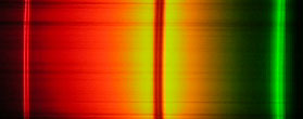 |
 |
For an explanation of why some spectral lines appear curved, click here.
For Color Spectrum photographs taken with a high quality small spectroscope, click
here.
For Color Spectrum photographs taken with a toy spectroscope, click here.
To see some of the lamps that produced these spectra, click here.